OilCalcsPro version 1.4.1 for Android adds additional capability!

Today a new version of OilCalcsPro for Android (version 1.4.1) was published.

The new version contains additional functionality as requested by some of our users, as well some improvements and bugfixes:

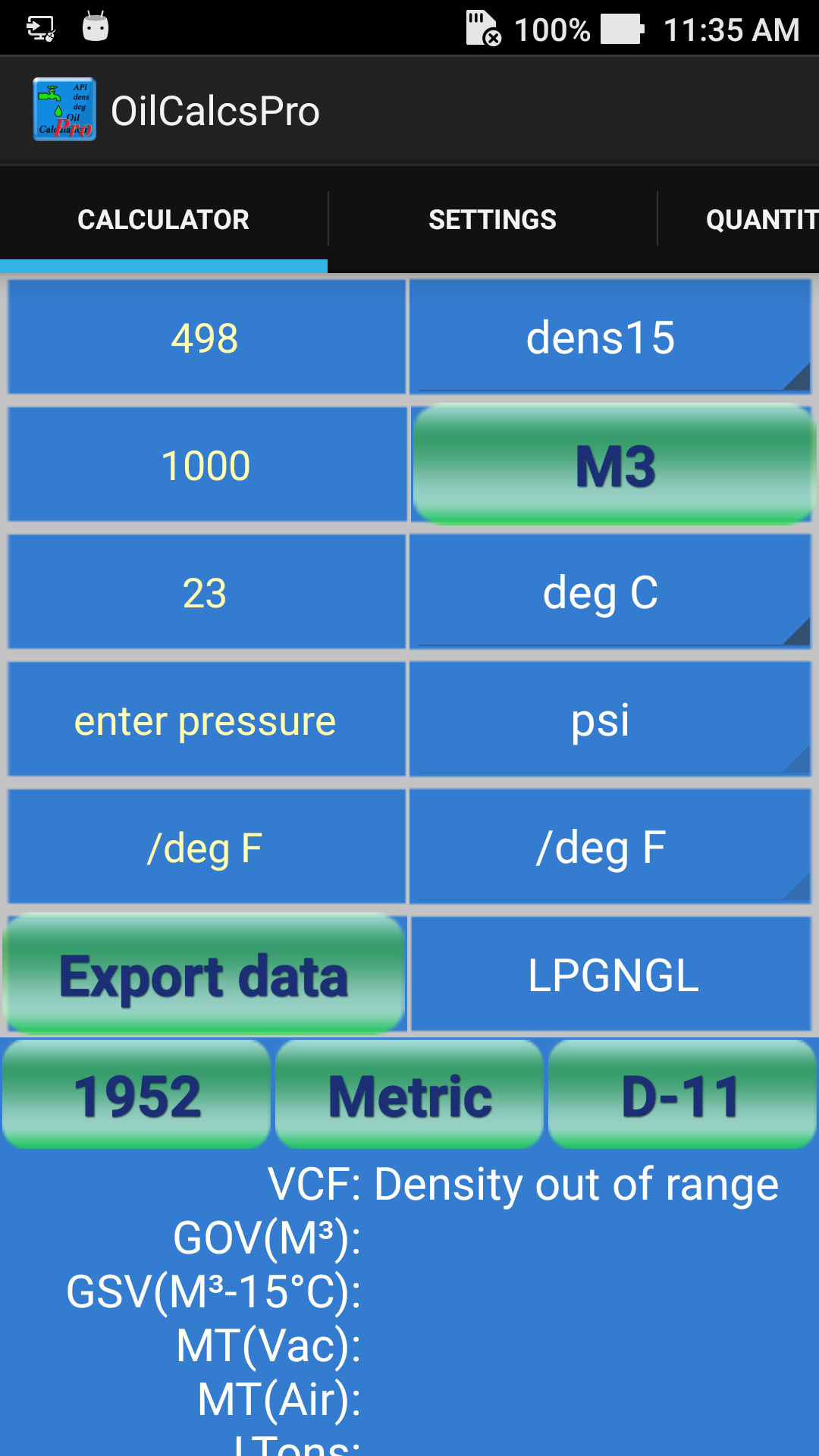
– Added the ability to choose between entering a thermal expansion coefficient (alpha) and a density correction factor when working with ‘Special applications’ such as MTBE, if for example no thermal expansion coefficient is known: in various ports around the world when dealing with products such as MTBE, a density correction factor (in /deg C) is provided instead of a thermal expansion coefficient. To enable calculating VCF, volumes and weights in that case, an additional field ‘density correction’ is now provided when selecting ‘Special applic’ as cargo type:

Using density correction to calculate weights & volume.

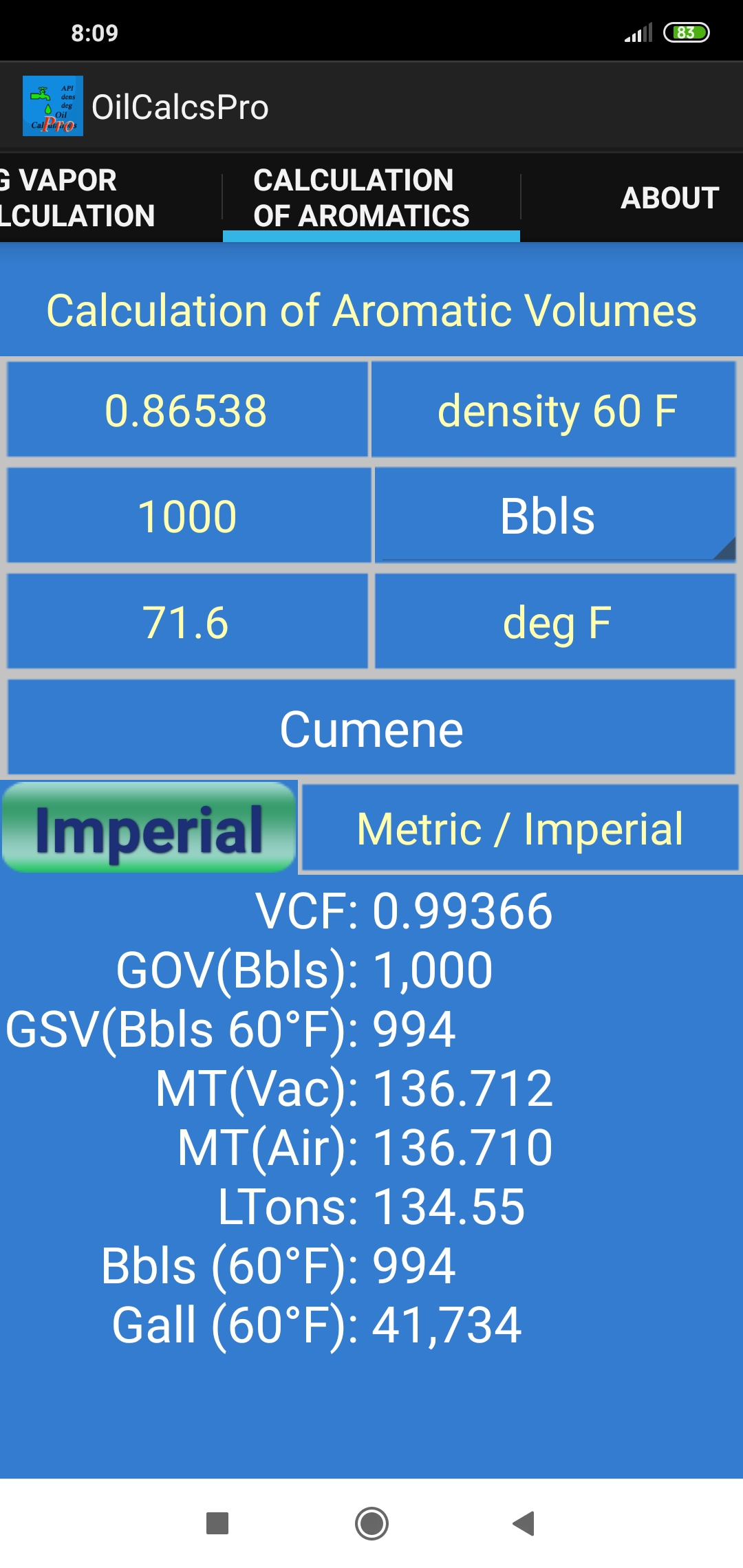
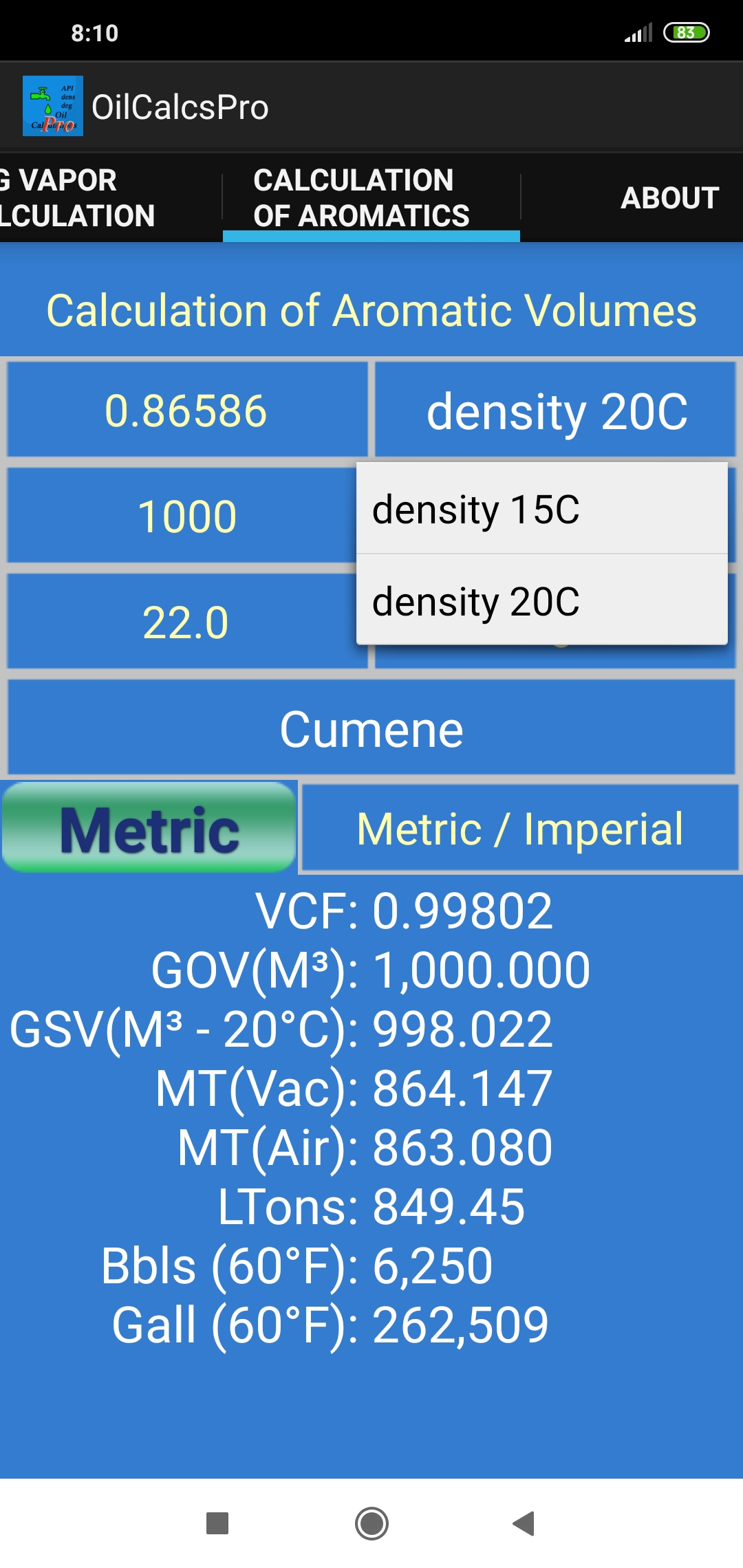
– Reverse calculation, for example from MTons in vacuum to all other units is also possible. In the main calculator screen the various calculations differ depending on whether density at 20°C or 15°C is used. In SI Metric mode when using relative density, observed density or API, the density value is internally converted to density at 15ºC and a GSV in M³ at 15ºC; when using density at 20ºC, the resulting GSV is at 20ºC. When in Imperial mode, all densities are converted internally to relative density and a GSV in M³ at 60°F. For the calculation of ‘Special applications’ the calculation methods are also split between using density at 15 and density at 20°C.

Calculating all weights * volume from MTV

– Updated the Quantity Editor to reflect the changes made in the main calculator screen:

Editing loaded report in the quantity editor

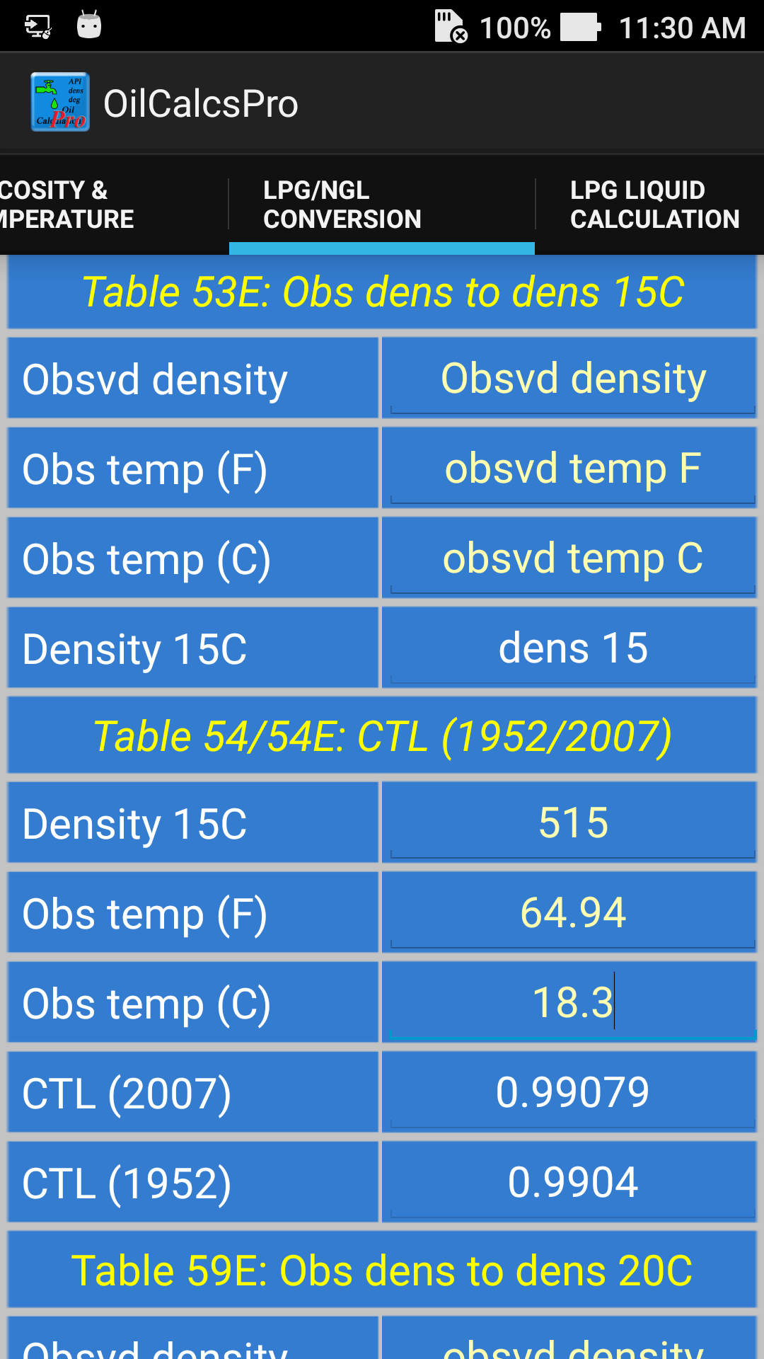
– The oil conversion screen has been updated to include calculations for ‘Special applications’ wherever possible: this was not yet the case for all conversion tables. The following tables are available: 5, 6, 23, 24, 53, 54, 59, 60, 4, 8, 9, 10, 11, 12, 13, 14, 52, 56, 57, 58. The calculations used are all basis API MPMS 2004 version (with 2007 amendments).

Table 6 all values

table58

tables5-8

tables9-14

tables52-58

In the Aromatics calculator a bug prevented displaying the two groups of Aromatic HydroCarbons using the temperature in °F when using Imperial mode: this has now been corrected.

The instruction manual has been updated and can be downloaded from the page in this blog with the title ‘User Manuals for Oil Calculators’.

The latest version can be downloaded from Google Play here:

OilCalcsPro version 1.4.0 for Android published!

Today a new version of OilCalcsPro for Android (version 1.4.0) was published.

The new version contains various updates and improvements:

– Added a new module, for calculating aromatics in accordance with ASTM D1555 and D1555M.

– Changed the way Bbls at 60°F are calculated when using density at 20°C to more accurately match the conversion from M³ at 20°C to Bbls at 60°F.

– Updated the Quantity Editor to reflect the changes made in the main calculator screen.

The calculation of aromatics uses ASTM D1555 to calculate VCF as well as weights and volumes using Imperial Standards, while D1555M uses SI Metric standards. To use this module, simply follow these steps:

1:Set SI Metric or Imperial Standards using the button ‘Metric’: by default the aromatics calculator uses the SI Metric Standard. When you press the ‘Metric’ button, the button title changes to ‘Imperial’, indicating that calculations are performed using the Imperial Standard:

 

2:Select the aromatic product you wish to calculate for, using the drop down (showing ‘Benzene’ by default):

3:When using the SI Metric Standard, select either ‘density 15C’ or ‘density 20C’:

4:When using the Imperial Standard, select either ‘Gallons’ or ‘Bbls’ as volume unit:

5:When you select an aromatics product, a default density corresponding to the selected product is automatically entered in the density field. If your density is different, simply update the density field.

6:VCF is calculated using either 4 or 5 decimals, depending on whether you have chosen to use 1980 tables or 2004 tables in ‘Settings’.

The instruction manual has been updated and can be downloaded from the page in this blog with the title ‘User Manuals for Oil Calculators’.

The latest version can be downloaded from Google Play here:

New Android app – Visco Temp(for free from 21st until 28th June)

Yesterday we published ‘Visco Temp’ on Google Play.

This is another standalone version of the same utility included in Oil Calculator Pro.

The visco temp app calculates (for fuel oils) an alternative temperature at a given viscosity or an alternative viscosity at a given temperature, on the basis of an initial viscosity and temperature, or on the basis of two sets of (viscosity, temperature) data.

Starting today 21st June Visco Temp is available for download for free until 28th June, thereafter it will be available at its regular price of USD 2.

 

NOTE: THIS APP HAS BEEN REMOVED IN ORDER TO COMPLY WITH GOOGLE PLAY POLICIES

You can download ‘Visco Temp’ here.

 

Visco Temp uses two methods to calculate alternative temperature and viscosity: the ‘V50’ formula and the ‘Walther’ equation. Depending on which method is used, a graph is drawn upon entering the required inputs, and there are fields available for entering an alternative viscosity and temperature, which when entered with data will give the resulting temperature or viscosity:

Available controls and fields:

Temperature toggle buttons:

The temperature can be entered in either °Celsius or °Fahrenheit, depending on the state of the toggle buttons. There are three areas where the user can enter temperature and in each area the temperature unit can be set independently. When the user toggles the button, any existing values are automatically converted.

 

Viscosity fields:

The viscosity is entered in centi Stokes (cSt). The upper half of the screen is basically divided into two portions: one portion for using the ‘V50’ formula, which is marked by ‘Using one reference only’, and one portion for using the ‘Walther’ equation, which is marked by ”Walther equation (using 2 reference points’)’.

 

Visco Limit:

The maximum viscosity displayed in the graph can be set using this button. When pressed, a list of possible viscosities shows up (500, 1000 etc) and once the user presses the desired limit, the graph is updated accordingly:

 

Show V50:

This is a toggle button that switches between displaying the graph using the V50 formula and the Walther equation. If no data is present in the V50 area, the graph will not show, and likewise for the Walther area.

 

Options menu:

The options menu (in the upper right hand corner of the screen on newer phones), allows the user to go to the ‘About’ screen, and also it allows the user to set the ‘theme’ for the graph. There are six possible themes, 3 with a black background and 3 with a white background:

 

Example – V50 formula:

If we enter a temperature of 50 °C and a viscosity of 380 cSt in the V50 area, as shown in the above picture, and then enter a temperature of 35 °C in the alternative temperature field (below the second temperature toggle button) we can see that the corresponding viscosity is  1089.8 cSt. Conversely if we would enter a viscosity of 200 cSt, we will see that the corresponding temperature is 60.9 °C.

Example – Walther equation:

If we enter a temperature of 38°C and a viscosity of 800 cSt for T1 and V1, and a temperature of 60°C and a viscosity of 200 cSt for T2 and V2, as shown in the above picture, and then enter a temperature of 50 °C in the alternative temperature field (next to the third temperature toggle button) we can see that the corresponding viscosity is  357 cSt. And if we enter a viscosity of 380 cSt, we will see that the corresponding temperature is 49 °C.

 

You can download ‘Visco Temp’ here.

 

New version of OilCalcsPro for Android launched!

Today a new version of OilCalcsPro for Android (version 1.2.1) was launched.

The new version contains various updates and improvements:

– Added three buttons in the calculator screen in order to change settings without having to go to the settings screen.

– Optimized various calculations to make the app respond faster.

– Revamped the user interface, with a new color theme.

– Added LPG table 54 (1952) as requested by users.

– Added both LPG table 54 (1952) and 54E (2007) in the LPG/NGL conversion screen.

– Added informative warning messages in calculator screen for temperature or density out of range.

New buttons in the calculator screen: these can be used to change between:

– Imperial and Metric units

– 1980 (1952 for LPG table 54) and 2004/2007 table versions

– Using table 56 or density – 11 points

Three buttons added in calculator screen

Using LPG table 54 (1952)

Table 54 and 54E added to LPG/NGL conversion screen

Out of range warning for density

Out of range warning for temperature

The instruction manual has been updated and can be downloaded from the page in this blog with the title ‘User Manuals for Oil Calculators’.

The latest version can be downloaded from Google Play here:

OilcalcsPro for desktop 101 – Part 4

In our last post concerning OilcalcsPro for desktop 101 we discussed some more calculations using the main calculator.

We also talked about the two simple fuel blenders, the problems encountered when loading two components of different temperature and density and the shrinkage caused by mixing two components with different densities. And finally we discussed how the viscosity blender works.

In today’s tutorial we are going to talk about the following topics:

• The visco – temp converter

• LPG/NGL calculations – liquid

• LPG/NGL calculations – vapor

If you are interested in following the examples on your own machine, the latest version of OilcalcsPro For Desktop can be downloaded here.

If you want to convert the demo version to the permanent pro version, buy a license code voucher here: Goto Paypal

So let’s get started with the visco – temp converter: to get to it click ‘Tools’ in the main screen, then click ‘Viscosity/temp conversion’ in the tools screen.

This utitility does the following things:

• For a given temperature / viscosity combination it calculates and displays the viscosity/temperature graph using the ‘V50’ formula.

• For two pairs of temperature and viscosity it calculates and displays the viscosity/temperature graph using the ‘Walthers equation.

• For a given viscosity it will calculate the corresponding temperature, either using the V50 formula or the Walthers equation.

• For a given temperature it will calculate the corresponding viscosity, either using the V50 formula or the Walthers equation.

The viscosity is in cSt, the temperature can be either in degrees Celsius or Fahrenheit.

Looking at the below screenshot, let’s have a look at the various controls:

V50 graph

In the top left corner you can see the V50 calculator: only one viscosity and one temperature are entered to enable displaying the graph. In the V50 calculator is a button that shows ‘°C’. If you press it, the temperature values will automatically be converted to degrees Fahrenheit, and you can then also enter your temperature values in degrees Fahrenheit. After converting to degrees Celsius, the temperature button now shows the text ‘°F’, and if you click it again, temperatures will be converted from degrees Fahrenheit back to Celsius.

Download dropbox for free

The viscosity and the temperature field in the top are the ones used to calculate the V50 graph. Below that are two more fields for viscosity and temperature; if you enter an alternative viscosity, the corresponding temperature is calculated and displayed in the second temperature field. Likewise if you enter an alternative temperature, the corresponding viscosity is calculated and displayed in the second viscosity field.

For a practical example, enter a value of 380 cSt and 50°C in the two fields in the top. As soon as you enter the values, the graph is automatically drawn. Above the graph there is a drop-down field where you can choose the maximum viscosity value to be plotted in the graph, and there is a button that presently says ‘Graph – single reference’. Clicking this button lets you switch between showing the V50 and the Walther graph.

Below the graph there is a check-box  that says ‘switch graph automatically when switching between Walther and V50; by default the check-box is ticked, so that when you enter a new value in the V50 calculator, automatically the V50 graph is drawn, and if you enter a new value in the Walther calculator, automatically the Walther graph is drawn and displayed.

Now if you enter a value of 500 in the alternative viscosity field, the temperature field will show 45.8°C. Conversely, if you enter a value of 49 in the alternative temperature field, the viscosity field will show 405 cSt. By default the viscosity range drop down is set at 500 cSt. If you change it to for example 1000 cSt, the graph is redrawn and the viscosity and temperature axis are both automatically adjusted.

Now lets make an example using the Walther equation: the Walther formula is usually written as: log_10*log_10*(ν_cS+a) = log₁₀(log_10*b+1/T^c). Using two sets of viscosity and temperature values, a and b can be solved and hence the graph can be calculated and plotted. Let’s enter the following values in the Walther calculator:

• 950 cSt at 18°C

• 120 cSt at 100°C

In below screenshot the graph is plotted for these values; if you now enter an alternative temperature of 50°C, you will see a calculated viscosity of 364.1 cSt for the corresponding viscosity:

Walther graph

By changing the viscosity range value in the drop down field, you can force the y-axis to a different viscosity maxima, with a maximum of 4,000 cSt.

Please note that while the V50 formula is good enough for a quick and easy approximation, it is not quite as accurate as the Walther formula. The V50 formula provides a reasonable estimate for viscosity / temperature conversions in the temperature range between approximately 30 °C and 120 °C for well known bunker fuels such as RMG 380.

If you need an accurate estimate for any fuel, definitely the Walther formula is the recommended one to use.

Next up is the LPG/NGL liquid calculation: this calculator can be used to calculate weights and volumes of a known quantity of LPG or NGL in a shore tank or ship tank.

To get there, click ‘Return’ on the visco/temp converter, and then in the tools screen, click the ‘LPG/NGL Calculation – Liquid.

To calculate the quantity of LPG or NGL, the following parameters are required:

• Relative density at 60°F or density at 15°C

• Liquid temperature

• Shrink factor of the tank

• Observed liquid volume

If you enter the relative density, this will automatically be converted to density at 15°C. This density will be used to calculate the CTL, using the calculations as described in API MPMS 11.2.4 (ASTM Technical Publication TP27).

The shrink factor is assumed to be 1 if no entry is made. Normally, the tank tables for the tank in question will provide the shrink factor, based on the liquid observed temperature.

Table 56 for conversion of weight in vacuo to air is calculated using:

T56 = (1 – (1.2 / dens15)) / (1 – (1.2 / 8100)).

After entering also the observed volume in M³, weight in vacuo and air are calculated using T56.

Now let us carry out an example: enter a relative density of 485, a liquid temperature of -15°C, a shrink factor of 0.99858 and an observed volume of 500 M³. You will see the density at 15°C is 485.4, the CTL is calculated at 1.08970 and T56 is calculated at 0.99768.

The resulting weight in vacuo is 264.095 MT, and the resulting weight in air is  263.481 MT.

The LPG/NGL calculator – vapor works a bit differently: in order to calculate the density of the vapor, the following formula is used:

d15= (288.15 * absPx * MolWeight) / (liqTemp * atmPx * 23.6382)

Where:

• d15 is vapor density at 15°C

• absPx is the absolute tank pressure in kPa

• MolWeight is the molecular weight of the vapor, approximately 44 for LPG and depending on the specific composition. For LNG (or NGL as it is also referred to), the molweight is approximately 18, again depending on the actual composition.

• liqTemp is the observed liquid temperature in °C

• AtmPx is the atmospheric pressure in kPa

Both the molecular weight and density at 15°C are normally provided with the quality certificate, but the density can also be calculated using for example the revised Klosek-McKinley method. That is however a topic worthy of an entire blog post in itself.

Let us now do an example: head over to the LPG/NGL vapor calculator by first clicking ‘Return’ inside the LPG/NGL liquid calculator, then click the ‘LPG/NGL calculator – vapor’ in the tools screen.

Assume the following values:

• Vapor temperature: -135°C

• Tank vapor pressure: 5.6 kPa

• Atmospheric pressure: 101.3 kPa

• Molecular weight: 16.5

• Vapor observed volume: 200 M³

• Shrink factor: 0.99954

The vapor density is calculated as 1.433 and the resulting weight in vacuo is 286.468 Kg (not MT!).

Well, we have come to the end of this tutorial! In the next tutorial we will talk about the following topics:

• LPG density calculation

• LPG/NGL conversions

• Oil conversions

If you are interested in following the examples on your own machine, the latest version of OilcalcsPro For Desktop can be downloaded here.

If you want to convert the demo version to the permanent pro version, buy a license code voucher here: Goto Paypal.