OilCalcsPro version 1.4.1 for Android adds additional capability!

Today a new version of OilCalcsPro for Android (version 1.4.1) was published.

The new version contains additional functionality as requested by some of our users, as well some improvements and bugfixes:

– Added the ability to choose between entering a thermal expansion coefficient (alpha) and a density correction factor when working with ‘Special applications’ such as MTBE, if for example no thermal expansion coefficient is known: in various ports around the world when dealing with products such as MTBE, a density correction factor (in /deg C) is provided instead of a thermal expansion coefficient. To enable calculating VCF, volumes and weights in that case, an additional field ‘density correction’ is now provided when selecting ‘Special applic’ as cargo type:

Using density correction to calculate weights & volume.

– Reverse calculation, for example from MTons in vacuum to all other units is also possible. In the main calculator screen the various calculations differ depending on whether density at 20°C or 15°C is used. In SI Metric mode when using relative density, observed density or API, the density value is internally converted to density at 15ºC and a GSV in M³ at 15ºC; when using density at 20ºC, the resulting GSV is at 20ºC. When in Imperial mode, all densities are converted internally to relative density and a GSV in M³ at 60°F. For the calculation of ‘Special applications’ the calculation methods are also split between using density at 15 and density at 20°C.

Calculating all weights * volume from MTV

– Updated the Quantity Editor to reflect the changes made in the main calculator screen:

Editing loaded report in the quantity editor

– The oil conversion screen has been updated to include calculations for ‘Special applications’ wherever possible: this was not yet the case for all conversion tables. The following tables are available: 5, 6, 23, 24, 53, 54, 59, 60, 4, 8, 9, 10, 11, 12, 13, 14, 52, 56, 57, 58. The calculations used are all basis API MPMS 2004 version (with 2007 amendments).

Table 6 all values

table58

tables5-8

tables9-14

tables52-58

In the Aromatics calculator a bug prevented displaying the two groups of Aromatic HydroCarbons using the temperature in °F when using Imperial mode: this has now been corrected.

The instruction manual has been updated and can be downloaded from the page in this blog with the title ‘User Manuals for Oil Calculators’.

The latest version can be downloaded from Google Play here:

OilCalcsPro version 1.4.0 for Android published!

Today a new version of OilCalcsPro for Android (version 1.4.0) was published.

The new version contains various updates and improvements:

– Added a new module, for calculating aromatics in accordance with ASTM D1555 and D1555M.

– Changed the way Bbls at 60°F are calculated when using density at 20°C to more accurately match the conversion from M³ at 20°C to Bbls at 60°F.

– Updated the Quantity Editor to reflect the changes made in the main calculator screen.

The calculation of aromatics uses ASTM D1555 to calculate VCF as well as weights and volumes using Imperial Standards, while D1555M uses SI Metric standards. To use this module, simply follow these steps:

1:Set SI Metric or Imperial Standards using the button ‘Metric’: by default the aromatics calculator uses the SI Metric Standard. When you press the ‘Metric’ button, the button title changes to ‘Imperial’, indicating that calculations are performed using the Imperial Standard:

 

2:Select the aromatic product you wish to calculate for, using the drop down (showing ‘Benzene’ by default):

3:When using the SI Metric Standard, select either ‘density 15C’ or ‘density 20C’:

4:When using the Imperial Standard, select either ‘Gallons’ or ‘Bbls’ as volume unit:

5:When you select an aromatics product, a default density corresponding to the selected product is automatically entered in the density field. If your density is different, simply update the density field.

6:VCF is calculated using either 4 or 5 decimals, depending on whether you have chosen to use 1980 tables or 2004 tables in ‘Settings’.

The instruction manual has been updated and can be downloaded from the page in this blog with the title ‘User Manuals for Oil Calculators’.

The latest version can be downloaded from Google Play here:

Cargo Surveyor for Android – Tutorials part 7: Ullage report – generating the pdf or jpg

The tutorials part 7 for the Android version of Cargo Surveyor is the second session of the Ullage report tutorial.

Recently we discussed in part the sixth document of the set of documents required to be produced in the load port, the ullage report.

Today we will discuss part 7 of the tutorials, which will deal with the remainder of the ullage report tutorial:

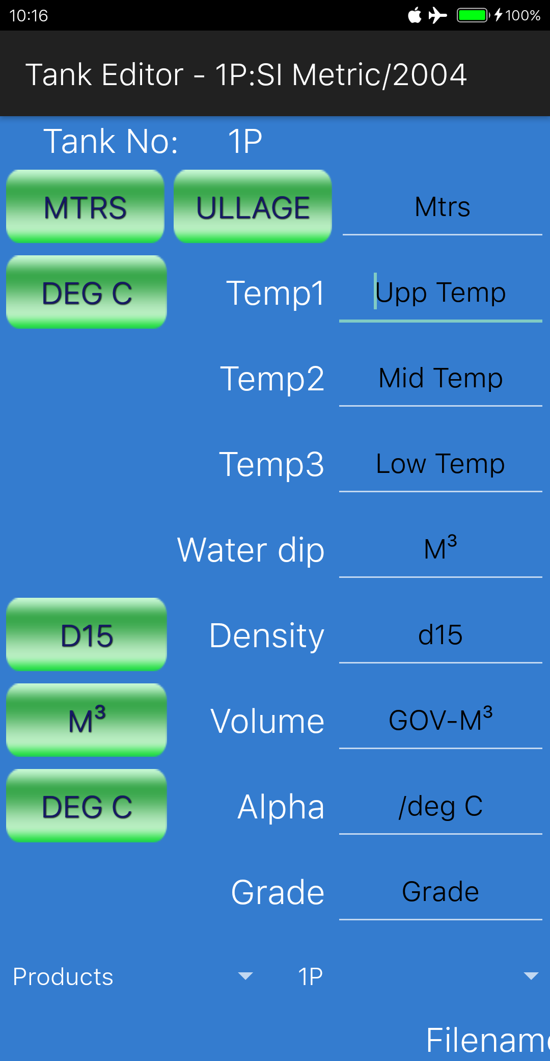
In the previous session concerning the ullage report we discussed how to enter data in the tank editor. We explained the function of the various buttons for changing units, and we discussed briefly the differences between the cargo types that are available. We will now discuss in more detail the use of the bottom line entries L1, L2 and L3 and we will enter all ullages for Testship upon completion of loading the 1st and 2nd parcel of mixed aromatics. After that we will show how to generate the ullage report, send it by mail and export it to csv.

First we will enter all data for the first ullage report. Let’s begin with saving a copy of the ullage report that we created in the last tutorial:

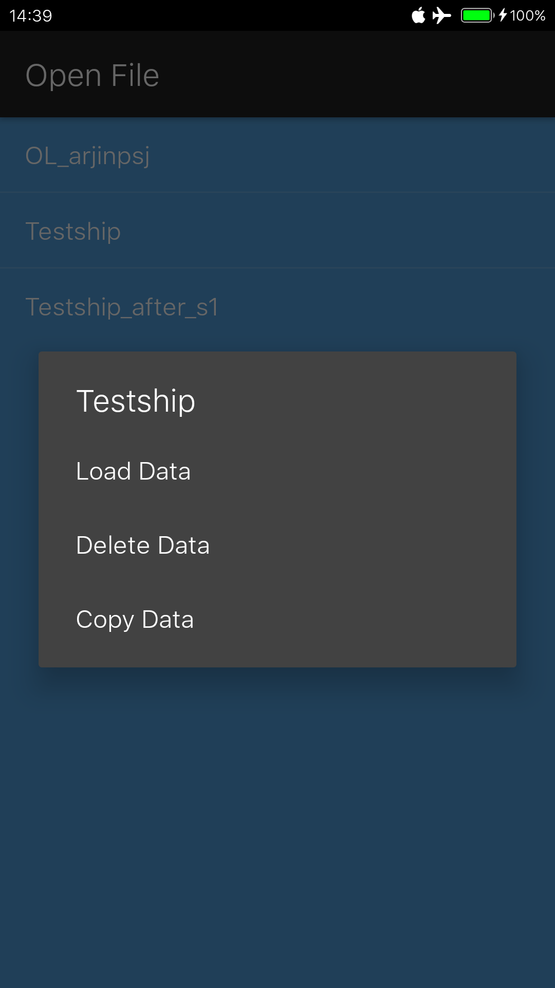
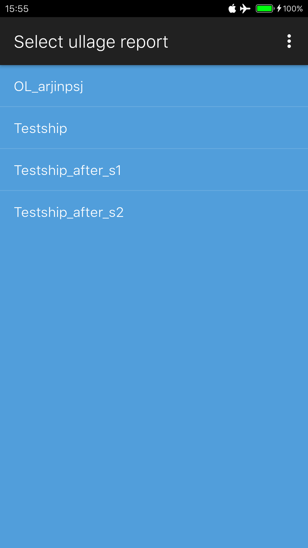
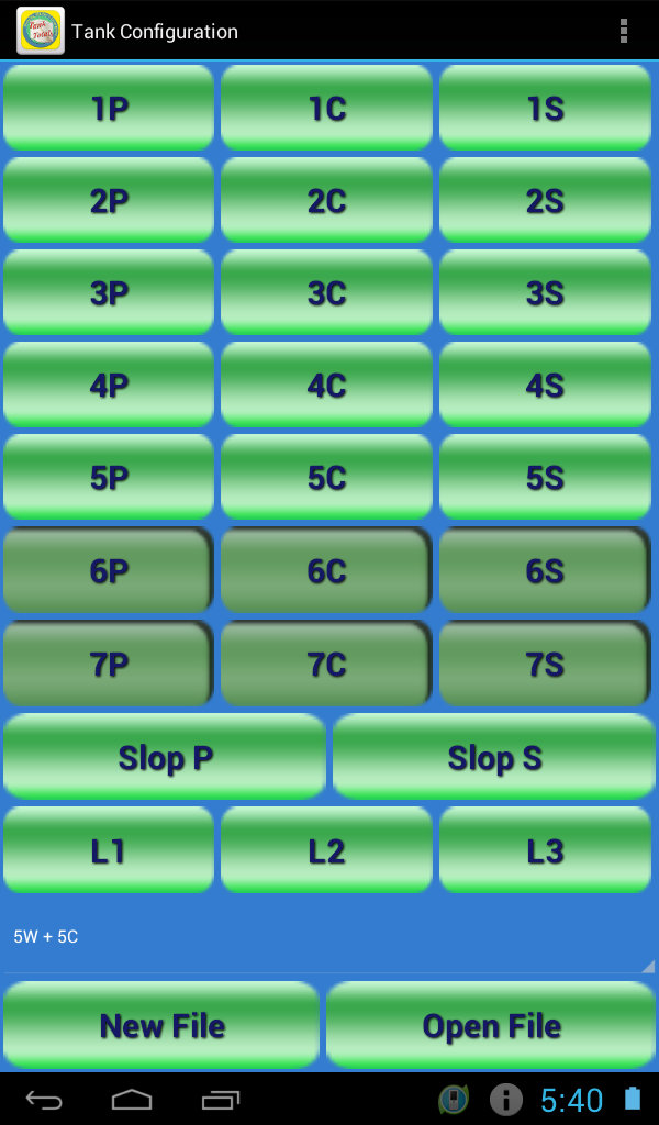
1: From the tank configuration screen, press ‘Open file’ and then press ‘Testship’ in the list of available ullage reports:

 

2: Press ‘Copy Data’ instead of ‘Load Data’; a copy of the original report is created, and let’s give the report the title ‘Testship after s1’. Any spaces entered in the file name will automatically be converted to underscores.

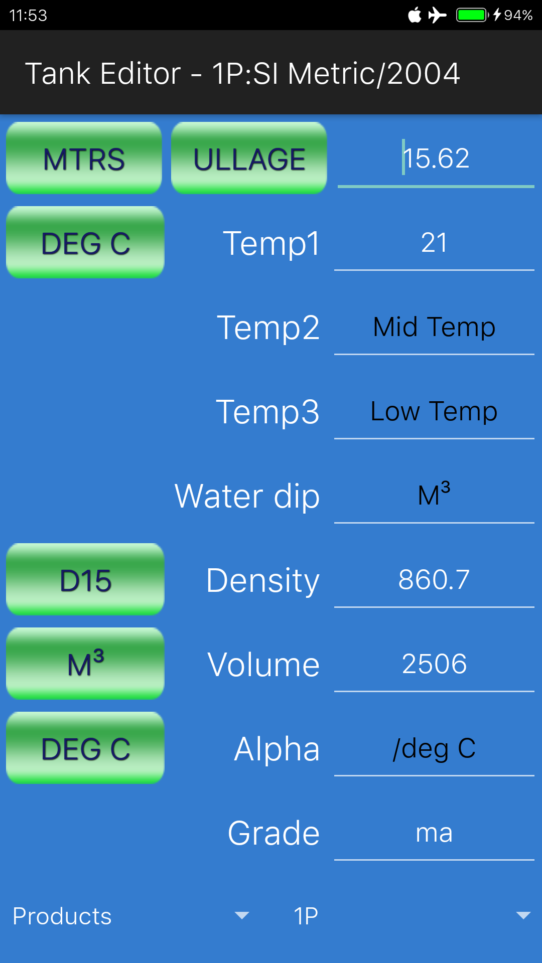
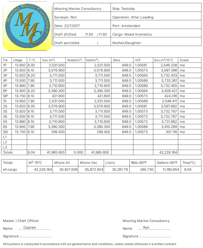
3: Now open ‘Testship_after_s1’ and fill in all the required data as shown below in the ullage report:

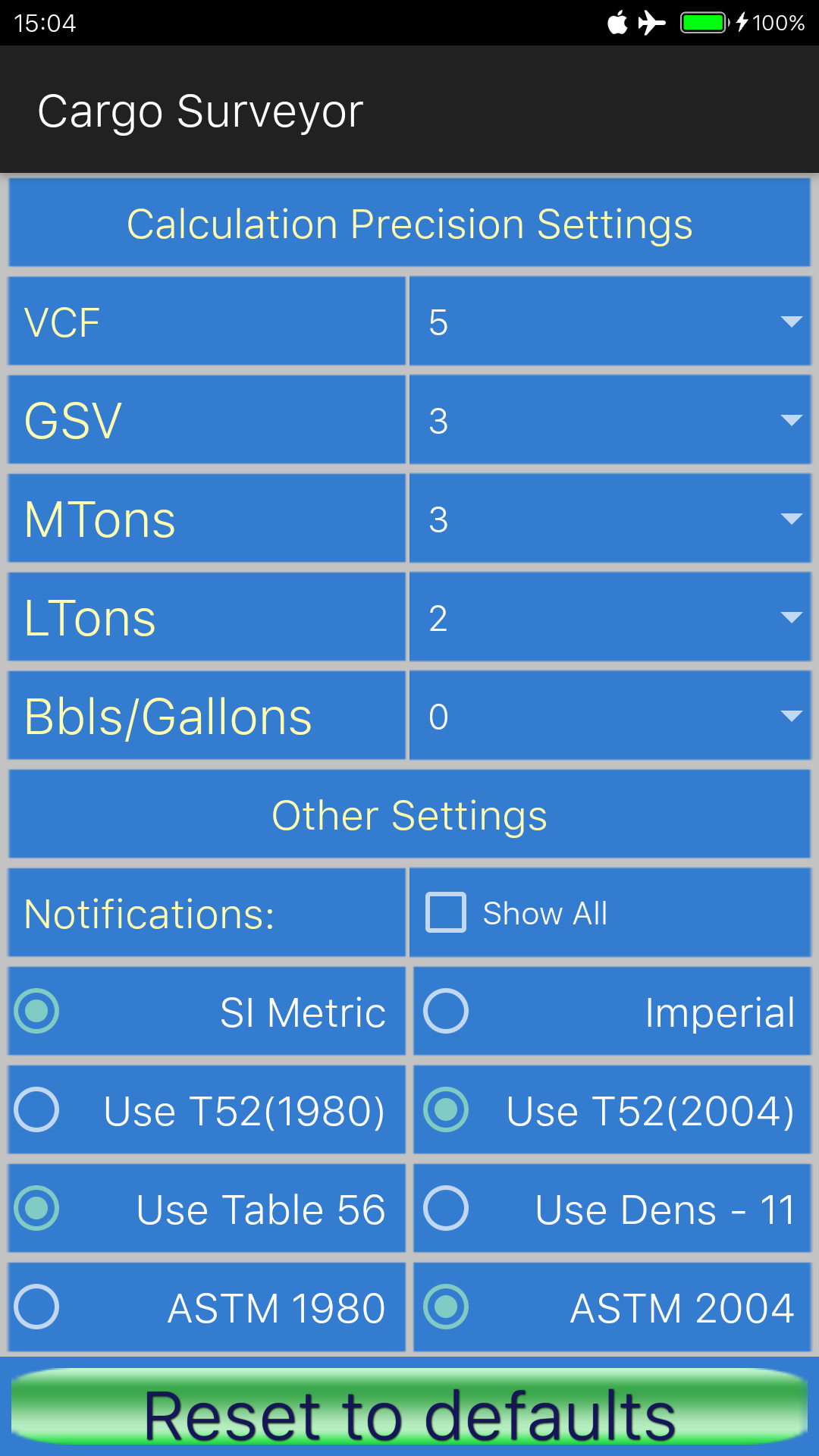
The density of the first parcel was 860.7 in vacuum, at 15 deg C, as supplied by the terminal. As discussed in one of the earlier tutorials, we are using ASTM tables 2004 version, with SI Metric settings.

If you do not get exactly the same figures as in the above report, the complete settings as used for our Testship are as follows:

You will have noticed that there are no entries for L1, L2 and L3; this vessel is fitted with deepwell pumps, and consequently has no bottom lines, so no quantities need to be added or deducted for bottom lines.

The use of bottom line entries is mostly applicable to VLCCs and SUEZ max vessels, where bottom line quantities tend to be big (around 300 M³ or more), and also to smaller size conventional tankers that are not fitted with deepwell pumps. Regardless of whether bottom lines are included in tank calibration tables or not, if the vessel carries more than one grade, and / or if not all tanks are used for loading or if one or more bottom lines remain empty after loading, the quantities to add or deduct to a grade due to bottom lines, need to be considered and entered accordingly in the ullage report.

In cases like our testship, where no bottom line quantities need to be entered, we could utilise L1, L2 and L3 for other tanks such as the Residual Oil Tank (if necessary).

Notice also that in pdf report settings we have changed the draft to 10.40 mtrs even keel upon completion of loading the first stage, and we have changed the setting of the ‘Before’ switch to ‘After’, to ensure that the ullage report shows ‘After loading’ instead of ‘Before Loading’.

Now let’s copy this ullage report into a new one, called ‘Testship after s2’, following the procedure as described above, and then we will open the newly copied ullage report in our tank editor and enter new ullages, volumes and density as shown in below ullage report.

Notice that in pdf report settings we have now changed the draft to 11.50 mtrs even keel upon completion of loading the second stage.

For the sake of convenience we will assume that all temperatures are still the same although in reality this is unlikely and we would normally do a full inspection including new temperatures. The new density is based on the mix by volume ratio of density of the first parcel (860.7) and the density of the second parcel (826.9):

Now that we have completed both ullage reports, we can have a look at how to generate the pdf / jpg, send it by email etc:

Upon completion of entering the data, after pressing the back button, we are back in the Tank Configuration screen. In the top right-hand corner of this screen there is an options menu, which if we press it, will shows links to ‘Current Totals’, ‘Settings’ etc and also ‘Pdf/jpg Reports’:

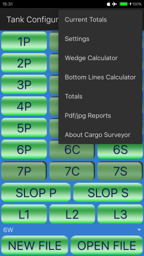
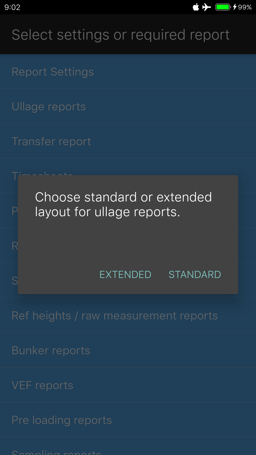
Pressing the link to ‘Pdf/jpg Reports’ will bring us to the Pdf reports section, where we can press on ‘Ullage Reports’ in order to generate our pdf or jpg image for the ullage report:

Now when we press ‘Ullage reports’, we will be presented with the list of available ullage reports:

As you can see, both ‘Testship_after_s1’ and ‘Testship_after_s2’ are in the list. If you press ‘Testship_after_s1’ you will be presented with the list of available grades within this report.

Normally there are always at least two entries in the list of grades: one entry called ‘TotalsAllGrades’, and one entry with a grade name that you have chosen when you created the ullage report. All existing grade names in the report will be listed here, and pressing a grade name will then produce an ullage report which will show only tanks containing that grade.

If you press ‘TotalsAllGrades’, the ullage report will show all tanks and a total cargo table, plus a breakdown of totals per grade. If you have entered only one grade, then there is no difference between selecting the grade name or selecting ‘TotalsAllGrades’, the report will be exactly the same.

So let us select the ‘ma’ grade. The first time you do this, the app will immediately show the pdf file (or the jpg image, more on that later) of the report as shown above. If later on you want to see the report again, the app will ask you ‘Entry exists, overwrite?’. If in the meantime you have made changes to the ullage report (changed ullages, or densities etc), then you need to select ‘OK’ and let the app overwrite the file.

After viewing the pdf or image file, if you press the back button, you will be asked if you want to send the ullage report by email; if you press ‘OK’ the app will then let you choose which email application to use (if you have more than one), and after selecting your preferred mail app, the mail composer shows up, with the pdf or jpg file already attached, and the subject of the mail entered as ‘Ullage Report (Pdf)’.

Also, if you have entered email addresses in the Pdf report settings, these addresses will already have been entered in the ‘To’ and ‘CC’ line. A maximum of 2 addresses will be entered in the ‘To’ line, and a maximum of 2 addresses will be entered in the ‘CC’ line. As you can see in the Pdf report settings screenshot below, a maximum of 4 email addresses can be entered automatically in the email. These addresses can either be entered manually, or be selected from your contacts. The first time you try to select addresses from your contacts the app will ask your permission to access your contacts.

After composing the email, it will either be sent to your outbox, or sent onto the web if you are connected and press the ‘send’ button in your email app. Once you close your email app, Cargo Surveyor will ask you if you wish to export the data to a csv file, and if you press ‘OK’ on that dialog, it will also ask you if you wish to send the csv file by email.

Both the pdf (or jpg) file and the csv file are stored on the internal storage of your phone. The pdf and the csv file can normally be found in the root of your internal storage. If you have opted to generate a jpg file (or if your phone runs an Android version lower than Kitkat – 4.4), a jpg file will be generated which will be saved in a directory called ‘saved_images’ in the root of your storage.

Cargo Surveyor will automatically detect if your phone is capable of generating pdf files, and will by default select the pdf format for reports if possible. If your phone is using an Android version below Kitkat 4.4, Cargo Surveyor will disable the choice between pdf and jpg, and will only produce jpg files.

What is the purpose of the csv (comma separated value) file? All the data inside the ullage report is put into a small text file, where each entry (this can be a number, or a combination of words) is separated from the next entry by a comma. This file can be opened by Microsoft Excel, and can be used to import the data from the ullage report into an excel spreadsheet. For advanced users it would also be possible to copy the exported csv file to another file (provided that you use the correct naming conventions etc) and generate a completely new ullage report from a desktop computer, which could then be imported to the phone by simply copying the csv file to the phone. More on that in a later tutorial.

In Cargo Surveyor this file is also used to backup and restore an ullage report (and most of the other reports can also make use of this). If you export an ullage report to csv, and wish to transfer the report to another phone where you also have Cargo Surveyor installed, all you have to do is copy the csv file to the other phone, and import the file into Cargo Surveyor on the other phone.

Another purpose is in case of corruption of the app, or if you completely uninstall the app and later want to re-install; if you have exported all your reports, it is very simple to import the csv files and have all your reports back with a minimum amount of effort.

We mentioned earlier in this tutorial the existence of an options menu in the top right-hand corner of the Tank Configuration screen; if you press the menu button and select ‘Current Totals’ while an ullage report has been loaded into memory, it will take you to a screen with the list of all grades within that ullage report and you can select a grade to view its totals.

Alternatively you can select the entry ‘Totals’ in the options menu, and select any existing ullage report, and then view for that selected ullage report its grand totals, or the totals for any grade:

Well, we have come to the end of tutorial no.7. In the next tutorial we will discuss the transfer executive summary.

In the mean time, for those who are interested in Cargo Surveyor for Android: the app can be downloaded here:

 

 

 

 

We post updates for the app in Google Play frequently to solve minor bugs, and advise all users to update as soon as a new update is available; we don’t use advertisements in Cargo Surveyor and we never will.

If you have any queries, suggestions, comments, criticism about the app or this blog post, please let us know! We always do our best to accommodate any requests for additions/modifications to our apps if they improve the value!

Cargo Surveyor for Android – Tutorials part 6: Ullage report – entering data in the editor

The tutorials part 6 for the Android version of Cargo Surveyor deals with the Ullage report.

Recently we discussed the fifth document of the set of documents required to be produced in the load port, the VEF report.

Today we will discuss part 6 of the tutorials, which will deal with the ullage report:

Cargo Surveyor is designed with user convenience and flexibility in mind. The app being used primarily on oil tankers and chemical tankers, we have chosen to give the user two different option sets regarding possible tank configurations:

• a standard layout, which accommodates a minimum of 12 tanks (5 pairs of wing tanks plus two slop tanks) and 3 bottom lines, and a maximum of 23 tanks (7 crosses plus two slop tanks) and 3 bottom lines.
• An extended layout, which accommodates a minimum of 34 tanks (16 pairs of wing tanks plus two slop tanks) and 3 bottom lines, and a maximum of 50 tanks (16 crosses plus two slop tanks) and 3 bottom lines.

The bottom lines and slop tanks can be used in any way the user wants to, they are simply considered as tanks just like the other tanks. (Not to be confused with actual bottom lines, which can either be included or excluded from tank tables). There are times however that the bottom lines L1, L2 and L3 are used to either add or deduct volume of cargo for a selected grade, and this depends indeed on whether bottom lines on the vessel are included in tank calibration tables or not, and what the grade of each bottom line is. More on this later.

When you open the app, the first screen that always appears is the layout selection screen, where you will be asked to choose between either the standard or the extended layout:

In the top right hand corner of this screen is also an options menu button, that will let you straight go to general settings etc.

For our testship, being a vessel with 6 pairs of wing tanks and 2 slop tanks (plus a residual oil tank), we will select the STANDARD layout. As soon as we press the button (‘USE STANDARD LAYOUT’) we are presented with the standard layout tank configuration editor:

At present only the ‘Open file’ button is enabled, all other buttons are disabled. If you previously created an ullage report than you can open that ullage report for editing by pressing the ‘Open file’ button and selecting the ullage report from the list of available reports. In our case we are going to create a new report from scratch so first we need to select the appropriate tank configuration; as soon as you press ‘Select tank configuration’, a pop up window appears where you can select a possible configuration. In these tank configurations slop tanks and bottom lines are not mentioned since they are always included:

For our testship we need to select ‘6W’: this will create an ullage report with 6 wing tanks + 2 slop tanks + 3 bottom lines. As soon as you press ‘6W’ on the drop down list in the above picture, you will notice that now all buttons 1-6P, 1-6S, Slop P, Slop S and L1, L2 and L3 buttons are enabled, as well as the ‘New File’ button.

We now press the ‘New File’ button; in the new window where we are asked to enter a file name, we can enter ‘Testship’ and press ‘OK’:

We are now taken directly to the tank editor (standard layout), with the new ullage report already created and opened and tank 1P selected:

Within the tank editor, the first thing we see in the top of the screen is 1P:SI Metric/2004. 1P is the name of the selected tank in the list of available tanks. SI Metric means that in general settings SI Metric units has been chosen, and 2004 indicates that ASTM 2004 tables have been selected.

There are five buttons on the screen for switching units (no.6 button ‘ULLAGE’ is only to indicate whether ullage or innage is being used, but presently this is not reflected in the actual report):

– ullage between meters and feet / inches: you can select this unit for each tank individually; this is handy in case the vessel has ullage tables using feet and inches while you want to make your report in metric units: first press the ‘MTRS’ button, so that the input changes to feet, inches. The title of the button now changes to ‘FT,IN’. Now enter the ullage (say for example ‘7, 8.5’). Now press the ‘FT,IN button again, and the ullage is automatically converted to 2.350 mtrs.

– temperature between deg C and deg F: same as with ullages, you can select the unit for each tank individually and convert between deg C and deg F with the press of a button, in this case the ‘DEG C’ button below the ‘MTRS’ button.

– density between density @ 15 deg C and API at 60 deg F: as with the other units, if you press the D15 button, the density (if you have entered one) will be automatically converted to API and the title of the button changes to ‘API’.

– volume between M³ and Bbls: likewise, if you press the M³ button, any volume you have entered will be converted to Bbls, and the title of the button will change to ‘BBLS’. Both volume in the volume field and the water dip field will be converted.

– thermal expansion coefficient (Alpha) between /deg C and /deg F: if you press the ‘DEG C’ button (below the M³ button), the expansion coefficient will be converted to /deg F.

All these units (except ullage) will be converted to the selected standard in the general settings when you generate the pdf report: if in general settings you have selected ‘SI Metric’, then all values will be printed in metric units, and if you have selected ‘Imperial’, then all values will be printed in imperial units.

Ullages however, will be printed depending on one particular setting in the pdf report settings: at the bottom of the pdf report settings there is an entry called ‘Keep ullages in original units’:

If this option is ticked, then ullages will be printed based on the ullage unit that has been used for the first tank: if the ullage of 1P is entered as ‘feet, in’ then all ullages will be printed in feet and decimal inches, regardless of whether you have selected metric or imperial units.

On the right hand side of the screen are fields to enter ullage, a maximum of three temperatures, the volume of any water in the tank, the density in vacuum at 15 deg C (or the API at 60 deg F), the tank volume, alpha (in case of special applications using table 54C or 6C and in case of chemicals), and the name of the grade.

If you have selected ‘Chemicals’ as cargo type, there is one additional field called ‘at temp’: here you can enter the temperature for the observed density (see below). Also the density button is disabled and will now have as title ‘DENSITY’ instead of ‘D15’. When chemicals is selected as cargo type, it is not possible to change the density unit to API.

At the bottom of the screen is the drop down to select the tank for which you want to enter data, currently pointing at 1P; to the left of the tank drop down is the cargo type selector, which you can set to either:

– Products

– Crude

– LubOil

– Special Applic(ations)

– Chemicals

If you select any cargo type except ‘Chemicals’, the ASTM tables are used for calculating the weights, VCF etc. In the case of Chemicals (not to confuse with ‘Special applications’) , the density is entered as observed density, together with a corresponding temperature for that density. In this case the ‘at temp’ and Alpha are used to calculate the actual weight in air. No GSV can be calculated since many chemicals such as FAME / vegetable oils are not even liquid at 15 deg C.

For all other cargo types the normal ASTM tables are used; which table is used for calculating the VCF depends on:

– The cargo type: if ‘Products’ is selected, either table 54B or 6B is used, if ‘Crude’ is selected, either table 54A or 6A is used etc.

– Whether in general settings ‘SI Metric’ or ‘Imperial’ has been selected; if Imperial is selected table 6B is used, if SI Metric is selected table 54B will be used. The same applies for Crude, LubOil and Special Applications.

Let us now enter an example referring to the screen shot below:

Testship will load the cargo of mixed aromatics in various stages, receiving parcels with different densities from different shore tanks.

Each parcel will be loaded evenly across all tanks so as to achieve a homogeneously commingled end product.

As can be seen in the picture on the left, we have entered an ullage of 15.62 mtrs, a temperature of 21 deg C, a density in vacuo at 15 deg C of 860.7, a volume of 2506 M³ and the grade name ‘ma’.

This grade name is arbitrary, you can enter any name you wish, as long as you ensure that this grade name is exactly the same for each tank carrying this grade, because the calculation of totals per grade is dependent on the grade name.

Now if you press the back button and return to the tank configuration screen, and then press the ‘1P’ button, you will see not only the info that we have just entered but also the VCF, GSV, MTons in air/vacuum, LTons, Bbls and Gallons are all displayed for this tank.

In the bottom of the screen the title of the report, as well as the grade name are displayed in an animated scrolling text field:

 

 

Phew! It has been a pretty long session already! We will take a break here, and discuss the remainder of the ullage report session in the next tutorial, part 7.

In the mean time, for those who are interested in Cargo Surveyor for Android: the app can be downloaded here:

 

 

 

 

We post updates for the app in Google Play frequently to solve minor bugs, and advise all users to update as soon as a new update is available; we don’t use advertisements in Cargo Surveyor and we never will.

If you have any queries, suggestions, comments, criticism about the app or this blog post, please let us know! We always do our best to accommodate any requests for additions/modifications to our apps if they improve the value!

Cargo Surveyor for Android – Tutorials part 2: OBQ report

The tutorials part 2 for the Android version of Cargo Surveyor deals with the OBQ report.

Recently we discussed the first document of the set of documents required to be produced in the load port, the pre-loading report.

Today we will discuss part 2 of the tutorials, which will deal with the OBQ report:

Upon completion of the tank inspection, we can enter our dips and wedge volumes in the OBQ report editor, and generate the report accordingly.

To get to the OBQ report editor we first need to go to the list of reports (‘Pdf/jpg Reports’), which can be accessed by pressing the options menu button (on newer phones this in the top right hand corner of the screen); this options menu is available from within:

• the first screen when you open the app
• the tank configuration screen for standard layout
• the tank configuration screen for extended layout

After pressing the option ‘Pdf/jpg Reports’, the list of available types of reports appears. If you accessed this from the very first screen, a message comes up first, asking you to confirm whether to use standard or extended layout for ullage reports. For OBQ reports you can choose either, it makes no difference. The choice between extended and standard layout is only important for ullage reports and transfer summary reports:

After selecting ‘EXTENDED’ or ‘STANDARD’ (if applicable), from the list above you select ‘ROB/OBQ reports’, and this will bring you to the list of available ROB/OBQ reports. If this is the first time that you are going to create a OBQ report, the list will show only one entry: ‘Create new entry’:

After pressing the ‘Create new entry’ line in the list, you will be asked to enter a title for the report, we can simply use our ‘Testship’ as title:

Once you press ‘OK’, the ROB/OBQ reports list shows the new entry ‘Testship’. The here described process for accessing the pdf/jpg reports, and for creating a new pdf/jpg report is the same for all the reports except for the ullage report and transfer report; the ullage report is created from within the STANDARD and EXTENDED tank layout. The transfer report is created based on the selection of two existing ullage reports. More on this in future tutorials.

Now if you select the ‘Testship’ entry, the OBQ reports editor appears if you select ‘Load/Edit data’ from the list of available actions:

When we first open this editor, ship name, port, date and cargo name will already have been filled in if we entered this information in the report settings, as discussed in part 1 of this tutorial.

We now first need to select whether this is an OBQ or an ROB report using the switch in the top of the editor (in the picture on the left the switch is already set to OBQ report). The difference between the two reports is that in OBQ report there is an entry for water dip / volume as well as for oil, whereas in the ROB report the entry for water dip/volume is missing.

Draft (in our example arrival drafts) and list if applicable can be entered, and we select either ‘Yes’ or ‘No’ for the question ‘Lines drained?’. Lines drained is actually not applicable for the OBQ report, it will be ignored in the actual report. It is only used for the ROB report.

Next down you can see the tank number drop down, which shows initially ‘1’. Below this tank drop down there is a drop down for choosing the innage units, either ‘Meters’ or ‘Ft, Inches’, and below that you can enter the tank name or number (such as ‘4C’, ‘1P’ etc). There is also a drop down for choosing between M3 and Bbls as volume unit. You can only switch between units when the first tank is selected.

You can either enter all tanks that were inspected, whether they were empty or not, or limit the report to tanks that actually contain OBQ. If you don’t fill in any information in the fields below the tank number drop down, and leave the tank name of the first tank as ‘1’, then the report will show just one line with tank data, and this line will simply be empty. The total amount of OBQ will also be shown as zero.

Alternatively you can make an entry for each individual tank and specify dips and wedge (or table) volumes as necessary. When you need to add a tank to the list, first make sure that you have given the desired name to the first tank, and then press the ‘+’ button.

A new entry will now be generated, which you can edit by selecting it in the drop down. In our current example, lets say that you named the first tank ‘1P’; as soon as you have changed the tank name on the first tank, this change will be reflected in the drop down, it will now show ‘1P’ instead of ‘1’. Now if you press the ‘+’ button, a message comes up saying ‘Tank (no. 2) added’. If you now press the drop down, you will see two entries in the list: ‘1P’, and ‘2’.

In order to edit the details for the 2nd tank, just press on ‘2’ in the list. If you had entered any details for the first tank, such as innage and wedge volume, these fields will now be empty and you can enter the correct data for this tank.

As you can see in the picture on the left, there are three fields for entering oil volume: Non liquid, Liquid(table) and Liquid(wedge). You only need to enter one liquid volume, either table or wedge. If you need the wedge volume you can press the ‘Wedge formula’ button to jump to the wedge formula tool to calculate the volume.

Below the entries for oil there are also two fields for water dip and volume.

You can mix table and wedge volumes for different tanks, the app will automatically calculate the totals of all three for all tanks. For each tank you also enter a remark if necessary.

Disclaimer text: if you have entered a disclaimer text in Report Settings, then that disclaimer will be used in the report instead of the disclaimer entered in the OBQ report editor.

An example of the completed OBQ report is shown here below:

 

This ends this tutorial. In part 3 we will discuss the Slop report.

In the mean time, for those who are interested in Cargo Surveyor for Android: the app can be downloaded here:

 

 

 

 

We post updates for the app in Google Play frequently to solve minor bugs, and advise all users to update as soon as a new update is available; we don’t use advertisements in Cargo Surveyor and we never will.

If you have any queries, suggestions, comments, criticism about the app or this blog post, please let us know! We always do our best to accommodate any requests for additions/modifications to our apps if they improve the value!

 

 

 

New version of OilCalcsPro for Android launched!

Today a new version of OilCalcsPro for Android (version 1.2.1) was launched.

The new version contains various updates and improvements:

– Added three buttons in the calculator screen in order to change settings without having to go to the settings screen.

– Optimized various calculations to make the app respond faster.

– Revamped the user interface, with a new color theme.

– Added LPG table 54 (1952) as requested by users.

– Added both LPG table 54 (1952) and 54E (2007) in the LPG/NGL conversion screen.

– Added informative warning messages in calculator screen for temperature or density out of range.

New buttons in the calculator screen: these can be used to change between:

– Imperial and Metric units

– 1980 (1952 for LPG table 54) and 2004/2007 table versions

– Using table 56 or density – 11 points

Three buttons added in calculator screen

Using LPG table 54 (1952)

Table 54 and 54E added to LPG/NGL conversion screen

Out of range warning for density

Out of range warning for temperature

The instruction manual has been updated and can be downloaded from the page in this blog with the title ‘User Manuals for Oil Calculators’.

The latest version can be downloaded from Google Play here:

OilcalcsPro for desktop 101 – Part 4

In our last post concerning OilcalcsPro for desktop 101 we discussed some more calculations using the main calculator.

We also talked about the two simple fuel blenders, the problems encountered when loading two components of different temperature and density and the shrinkage caused by mixing two components with different densities. And finally we discussed how the viscosity blender works.

In today’s tutorial we are going to talk about the following topics:

• The visco – temp converter

• LPG/NGL calculations – liquid

• LPG/NGL calculations – vapor

If you are interested in following the examples on your own machine, the latest version of OilcalcsPro For Desktop can be downloaded here.

If you want to convert the demo version to the permanent pro version, buy a license code voucher here: Goto Paypal

So let’s get started with the visco – temp converter: to get to it click ‘Tools’ in the main screen, then click ‘Viscosity/temp conversion’ in the tools screen.

This utitility does the following things:

• For a given temperature / viscosity combination it calculates and displays the viscosity/temperature graph using the ‘V50’ formula.

• For two pairs of temperature and viscosity it calculates and displays the viscosity/temperature graph using the ‘Walthers equation.

• For a given viscosity it will calculate the corresponding temperature, either using the V50 formula or the Walthers equation.

• For a given temperature it will calculate the corresponding viscosity, either using the V50 formula or the Walthers equation.

The viscosity is in cSt, the temperature can be either in degrees Celsius or Fahrenheit.

Looking at the below screenshot, let’s have a look at the various controls:

V50 graph

In the top left corner you can see the V50 calculator: only one viscosity and one temperature are entered to enable displaying the graph. In the V50 calculator is a button that shows ‘°C’. If you press it, the temperature values will automatically be converted to degrees Fahrenheit, and you can then also enter your temperature values in degrees Fahrenheit. After converting to degrees Celsius, the temperature button now shows the text ‘°F’, and if you click it again, temperatures will be converted from degrees Fahrenheit back to Celsius.

Download dropbox for free

The viscosity and the temperature field in the top are the ones used to calculate the V50 graph. Below that are two more fields for viscosity and temperature; if you enter an alternative viscosity, the corresponding temperature is calculated and displayed in the second temperature field. Likewise if you enter an alternative temperature, the corresponding viscosity is calculated and displayed in the second viscosity field.

For a practical example, enter a value of 380 cSt and 50°C in the two fields in the top. As soon as you enter the values, the graph is automatically drawn. Above the graph there is a drop-down field where you can choose the maximum viscosity value to be plotted in the graph, and there is a button that presently says ‘Graph – single reference’. Clicking this button lets you switch between showing the V50 and the Walther graph.

Below the graph there is a check-box  that says ‘switch graph automatically when switching between Walther and V50; by default the check-box is ticked, so that when you enter a new value in the V50 calculator, automatically the V50 graph is drawn, and if you enter a new value in the Walther calculator, automatically the Walther graph is drawn and displayed.

Now if you enter a value of 500 in the alternative viscosity field, the temperature field will show 45.8°C. Conversely, if you enter a value of 49 in the alternative temperature field, the viscosity field will show 405 cSt. By default the viscosity range drop down is set at 500 cSt. If you change it to for example 1000 cSt, the graph is redrawn and the viscosity and temperature axis are both automatically adjusted.

Now lets make an example using the Walther equation: the Walther formula is usually written as: log_10*log_10*(ν_cS+a) = log₁₀(log_10*b+1/T^c). Using two sets of viscosity and temperature values, a and b can be solved and hence the graph can be calculated and plotted. Let’s enter the following values in the Walther calculator:

• 950 cSt at 18°C

• 120 cSt at 100°C

In below screenshot the graph is plotted for these values; if you now enter an alternative temperature of 50°C, you will see a calculated viscosity of 364.1 cSt for the corresponding viscosity:

Walther graph

By changing the viscosity range value in the drop down field, you can force the y-axis to a different viscosity maxima, with a maximum of 4,000 cSt.

Please note that while the V50 formula is good enough for a quick and easy approximation, it is not quite as accurate as the Walther formula. The V50 formula provides a reasonable estimate for viscosity / temperature conversions in the temperature range between approximately 30 °C and 120 °C for well known bunker fuels such as RMG 380.

If you need an accurate estimate for any fuel, definitely the Walther formula is the recommended one to use.

Next up is the LPG/NGL liquid calculation: this calculator can be used to calculate weights and volumes of a known quantity of LPG or NGL in a shore tank or ship tank.

To get there, click ‘Return’ on the visco/temp converter, and then in the tools screen, click the ‘LPG/NGL Calculation – Liquid.

To calculate the quantity of LPG or NGL, the following parameters are required:

• Relative density at 60°F or density at 15°C

• Liquid temperature

• Shrink factor of the tank

• Observed liquid volume

If you enter the relative density, this will automatically be converted to density at 15°C. This density will be used to calculate the CTL, using the calculations as described in API MPMS 11.2.4 (ASTM Technical Publication TP27).

The shrink factor is assumed to be 1 if no entry is made. Normally, the tank tables for the tank in question will provide the shrink factor, based on the liquid observed temperature.

Table 56 for conversion of weight in vacuo to air is calculated using:

T56 = (1 – (1.2 / dens15)) / (1 – (1.2 / 8100)).

After entering also the observed volume in M³, weight in vacuo and air are calculated using T56.

Now let us carry out an example: enter a relative density of 485, a liquid temperature of -15°C, a shrink factor of 0.99858 and an observed volume of 500 M³. You will see the density at 15°C is 485.4, the CTL is calculated at 1.08970 and T56 is calculated at 0.99768.

The resulting weight in vacuo is 264.095 MT, and the resulting weight in air is  263.481 MT.

The LPG/NGL calculator – vapor works a bit differently: in order to calculate the density of the vapor, the following formula is used:

d15= (288.15 * absPx * MolWeight) / (liqTemp * atmPx * 23.6382)

Where:

• d15 is vapor density at 15°C

• absPx is the absolute tank pressure in kPa

• MolWeight is the molecular weight of the vapor, approximately 44 for LPG and depending on the specific composition. For LNG (or NGL as it is also referred to), the molweight is approximately 18, again depending on the actual composition.

• liqTemp is the observed liquid temperature in °C

• AtmPx is the atmospheric pressure in kPa

Both the molecular weight and density at 15°C are normally provided with the quality certificate, but the density can also be calculated using for example the revised Klosek-McKinley method. That is however a topic worthy of an entire blog post in itself.

Let us now do an example: head over to the LPG/NGL vapor calculator by first clicking ‘Return’ inside the LPG/NGL liquid calculator, then click the ‘LPG/NGL calculator – vapor’ in the tools screen.

Assume the following values:

• Vapor temperature: -135°C

• Tank vapor pressure: 5.6 kPa

• Atmospheric pressure: 101.3 kPa

• Molecular weight: 16.5

• Vapor observed volume: 200 M³

• Shrink factor: 0.99954

The vapor density is calculated as 1.433 and the resulting weight in vacuo is 286.468 Kg (not MT!).

Well, we have come to the end of this tutorial! In the next tutorial we will talk about the following topics:

• LPG density calculation

• LPG/NGL conversions

• Oil conversions

If you are interested in following the examples on your own machine, the latest version of OilcalcsPro For Desktop can be downloaded here.

If you want to convert the demo version to the permanent pro version, buy a license code voucher here: Goto Paypal.

 

 

Tank Totals Calculator for Android: update released

A few days ago MMC published a new version of Tank Totals Calculator (Version 1.0.7)

For an introduction video, see this link:  https://youtu.be/P7Lb2Wi1W3c

The new version comes with various bug fixes, and several improvements have been made:

• Inline conversion between Metric and Imperial units has been updated and is now completely fail safe.

• The soft keyboard has been reconfigured and now changes automatically when switching between Metric and Imperial units while at the same time only allowing the user to enter valid characters.

• All inputs have been given additional protection against invalid entries, so that crashes will not occur when entering invalid numbers etc.

• The settings screen and the wedge calculator are now available from the start up screen, it is not necessary anymore to first select a layout screen:

Settings & wedge Calculator on first screen

• The precision setting for Bbls is now also applied to US Gallons:

Settings screen

• In the previous version, when selecting extended layout, it was possible to select an invalid configuration under certain circumstances, which would cause the app to crash. The code for this section has been completely rewritten to ensure that this does not happen.

Download dropbox for free

The difference between the standard layout and the extended layout is that in the standard layout the user has a maximum of 7 crosses plus two slop tanks plus 3 bottom lines to chose from, whereas in the extended layout the user gets the same two slop tanks and 3 bottom lines, but can configure the number of wing tanks and center tanks as either zero or any number between 8 and 16.

In other words in the standard layout a maximum of 7 * 3 + 2 + 3 = 25 tanks / bottom lines can be used, whereas in the extended layout a maximum of 16 * 3 + 2 + 3 = 53 tanks / bottom lines can be used.

The way the tanks are presented for viewing individual tank data once the relevant information has been entered, is distinctly different for the extended layout compared to the standard layout:

In the standard layout, once the required data has been entered, and the user returns to the tank configuration screen, each tank can be selected for viewing all entered data and calculated parameters by pressing the button for that tank:

Selecting tankdata in standard layout

In the extended layout version however, the desired tank must be selected using the drop down list as shown in the screen below:

Select tank to view data

A detailed tutorial regarding the use of Tank Totals Calculator, as well as a full description of all functions and capabilities can be found elsewhere in this blog.

Tank Totals Calculator can be downloaded in the Google Play store here:

 For an introduction video, see this link:  https://youtu.be/P7Lb2Wi1W3c

Android Oil Calculator Pro – Important update released

MMC has released version 1.1.1 of Oil Calculator Pro today (12th November 2015).

The updated version can be downloaded in Google Play here.

 

For an introductory video on youtube, here is a link:   https://www.youtube.com/watch?v=CxM13B1eWPU

The update comes with various bug fixes, and a graphing utility has been added now to the Visco / Temperature converter:

Visco / Temperature converter

Graph for Walther equation

Graph for V50 equation

The graphing utility lets the user choose whether to view either the Walther graph or the V50 graph using the button ‘Show V50’. This text automatically changes to ‘Show Walther’ after selecting V50.

The graph is automatically adjusted for screen size, temperature and viscosity range, and the user can select which viscosity range he wants to use (i.e 0 – 500, or 0 – 1000 etc):

Select Viscosity range

There are different color themes available that the user can choose from:

Select color theme

Bugs that were fixed in this update:

• In various screens erroneous input (for example entering a ‘.’ in a density field) caused a crash. All functions have been updated with additional crash protection in the case of wrong / missing input.

• Some text fields showed a keyboard with minus sign when the input was supposed to be positive only. All such fields have been updated.

For those unfamiliar with Oil Calculator Pro, the app contains the following features:

• Calculation of volume correction factor, weights and volumes, both using SI Metric and Imperial units.

• Calculations can be performed using both ASTM tables 1980 and 2004.

• Reverse calculation using Metric Tons, Bbls 60F, GSV or Ltons as a starting point.

• Storing an unlimited number of weight/volume calculations in a data base. These calculations can later be retrieved, reviewed and edited.

• Oil conversions: convert between observed density, API, density 15ºC, density 20ºC and relative density.

• These conversions can also be done ‘inline’ in the calculator tab.

• Oil conversions: ASTM version 2004 of tables 5, 6, 23, 24, 53, 54, 59 and 60 are provided for lookup. Each table contains values for Products, Crude, Luboils and Special Applications (where applicable, i.e. table 6, 24, 54 and 60).

• LPG density calculator using the Francis formula.

• LPG / NGL conversions: provides lookup for table 23E, table 53E and 59E.

• LPG / NGL liquid and vapor calculations: calculate Mtons in vac and Mtons in air based on required inputs.

• Fuel blenders, for calculating shrinkage and resulting density, and to check which product to load first based on density and temperature.

• Viscosity blender: blending of up to 10 components, calculates resulting viscosity, density, pour point and flash point. The 10 components are stored in a database, and can be retrieved at any time for reviewing, editing etc.

• Viscosity fraction calculator: calculate fractions of 2 components for a target viscosity.

• Viscosity and temperature: contains two sections; one section using a modified V50 formula, to calculate either viscosity or temperature, based on a given viscosity and temperature. The other section  uses the Walther equation (i.e. two viscosities and two temperatures) to establish the graph, and calculate an alternative viscosity or temperature. This unit conforms with ASTM D341.

Download dropbox for free

More information on the various modules can be found elsewhere in this blog. For those interested in downloading:

The app can be downloaded in Google Play here.

 

Android Oil Calculator Pro – new version released

MMC has released version 1.1.0 of Oil Calculator Pro today (30th October 2015).

The updated version can be downloaded in Google Play here.

For an introductory video on youtube, here is a link:   https://www.youtube.com/watch?v=CxM13B1eWPU

 

The update comes with numerous bug fixes, the most important one being the updated quantity editor, which was causing the app to crash on several phones.

With the assistance of some of our customers we were able to finally trace the origin of this bug and implement a solution.

The app now checks whether a data file (named ‘dummy’) exists in the quantity editor. If this file does not exist it is automatically created.

The app will prevent deleting this file. The ‘dummy’ file can be used like any other data file created by the user.

Other bugs that were fixed in this update:

• In the Viscosity Blender, volume and density are now consistently saved in M³ and density 15ºC only, regardless of whether the unit setting is SI Metric or Imperial. When the user opens the last saved data, the data is converted and displayed in the units as selected in the settings screen so that users who wish to work with API and Bbls can do so by selecting ‘Imperial System’ in settings, and users who prefer to work with density and M³ can do so by selecting ‘Metric System’ in the settings tab.

• In the calculator tab, some inter conversions were not working properly (e.g negative API to density 15ºC). These have now been fixed.

• In the quantity editor, changing between API and density with no value in the field caused the app to crash, this is now fixed.

A future feature which is still being developed is the display of viscosity / temperature graphs for the Viscosity & Temperature tab. This will be added in the next update.

For those unfamiliar with Oil Calculator Pro, the app contains the following features:

• Calculation of volume correction factor, weights and volumes, both using SI Metric and Imperial units.

• Calculations can be performed using both ASTM tables 1980 and 2004.

• Reverse calculation using Metric Tons, Bbls 60F, GSV or Ltons as a starting point.

• Storing an unlimited number of weight/volume calculations in a data base. These calculations can later be retrieved, reviewed and edited.

• Oil conversions: convert between observed density, API, density 15ºC, density 20ºC and relative density.

• These conversions can also be done ‘inline’ in the calculator tab.

• Oil conversions: ASTM version 2004 of tables 5, 6, 23, 24, 53, 54, 59 and 60 are provided for lookup. Each table contains values for Products, Crude, Luboils and Special Applications (where applicable, i.e. table 6, 24, 54 and 60).

• LPG density calculator using the Francis formula.

• LPG / NGL conversions: provides lookup for table 23E, table 53E and 59E.

• LPG / NGL liquid and vapor calculations: calculate Mtons in vac and Mtons in air based on required inputs.

• Fuel blenders, for calculating shrinkage and resulting density, and to check which product to load first based on density and temperature.

• Viscosity blender: blending of up to 10 components, calculates resulting viscosity, density, pour point and flash point.

• Viscosity fraction calculator: calculate fractions of 2 components for a target viscosity.

• Viscosity and temperature: contains two sections; one section using a modified V50 formula, to calculate either viscosity or temperature, based on a given viscosity and temperature. The other section  uses the Walther equation (i.e. two viscosities and two temperatures) to establish the graph, and calculate an alternative viscosity or temperature. This unit conforms with ASTM D341.

Download dropbox for free

More information on the various modules can be found elsewhere in this blog. For those interested in downloading:

The app can be downloaded in Google Play here.